

STARBURST ENTERPRISE PERFORMANCE TUNING — A PRACTITIONER'S SERIES
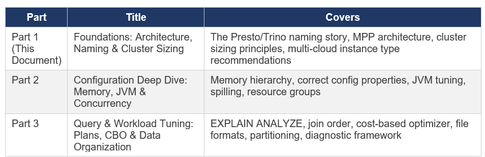
Part 1: Foundations — Architecture, Naming & Cluster Sizing

What sparked this series: A junior engineer on our team noticed that RAM utilization on our Starburst cluster was consistently above 80%, with all 25 worker nodes running at full capacity. Rather than raising an incident, I realised this was a teaching moment about how MPP query engines actually work and it became the foundation for this entire series of posts.
About This Series
This is a three-part practitioner series on Starburst Enterprise performance tuning. Each part is standalone but they build on one another. The series covers what I have learned deploying and tuning Starburst Enterprise in production, cross-referenced against official Starburst documentation (SEP 477-e LTS, November 2025) and the Presto/Trino Training Series.
Note: Everything in this series is based on my own production experience, combined with learnings from official Starburst and Trino documentation, along with other trusted resources. Wherever specific sources have influenced the content, I’ve credited them explicitly. This is not a copy of any documentation it’s my own interpretation, synthesis, and practical understanding of how these systems behave in real-world scenarios. If you notice anything that seems off or outdated, I genuinely welcome the feedback as this space evolves quickly, and there’s always more to learn.I really enjoyed putting this series together from start to finish. After completing the writing, I used ChatGPT to help refine the grammar and improve readability, while keeping my original thoughts and intent intact..
Chapter 1: The Naming Story — Presto, PrestoSQL, and Trino
Before any performance discussion, you need to understand the naming landscape. If you have read documentation, training slides, blog posts, and academic papers about this technology, you will have encountered ‘Presto’, ‘PrestoSQL’, ‘PrestoDB’, and ‘Trino’ used in ways that seem interchangeable but are not. This causes real confusion, so let me set the record straight.
1.1 Origins at Facebook (2012–2018)
Presto was created at Facebook in 2012 by four engineers Martin Traverso, Dain Sundstrom, David Phillips, and Eric Hwang as a replacement for Apache Hive. The problem they were solving was straightforward: Hive was too slow for the interactive analytics Facebook needed over its multi-petabyte Hadoop data warehouse. Facebook open-sourced the project in November 2013. Inside Facebook the project was called PrestoDB to distinguish it from unrelated projects.
1.2 The 2018-2019 Governance Disagreement and Fork
In late 2018, Facebook made a governance decision that the original creators considered incompatible with healthy open source community management: granting Facebook engineers commit access without the standard community merit process. The four founders left Facebook and in January 2019 forked the codebase, creating the Presto Software Foundation as an independent non-profit. Their fork was initially named PrestoSQL , the same software, same team, different governance.
1.3 The December 2020 Rename to Trino
In September 2019, Facebook transferred PrestoDB to The Linux Foundation, which also applied for and received a trademark on the name ‘Presto’. After extended negotiations between the communities, the PrestoSQL team was forced to rename. On December 27, 2020, PrestoSQL was officially renamed Trino. The community, codebase, and leadership remained identical only the name changed. Since the fork, Trino has seen approximately three times the development velocity of PrestoDB.
1.4 Where Starburst Fits
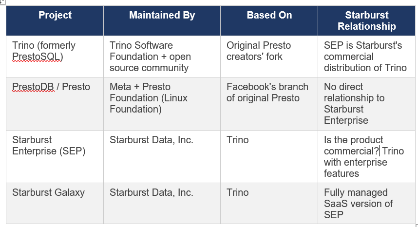
Note: When you see ‘Presto’ in Starburst training materials from 2020 (including the training series that informs much of this guide), that referred to what is now called Trino the same engine, same original authors, different name. The architecture, concepts, and configuration principles documented in those 2020 sessions remain fully valid for current Trino/Starburst Enterprise.
1.5 Why Starburst Documentation Still References ‘Presto’
You will still encounter ‘Presto’ references in Starburst’s own documentation, especially in older blog posts, some connector code, and historical training materials. This is because:
Content written before December 2020 legitimately referred to the engine as Presto (PrestoSQL)
The academic research paper ‘Presto: SQL on Everything’ (published by Facebook engineers, 2019) predates the rename and is universally cited by its original title.
Some third-party tools use the Presto JDBC driver or Presto SQL parser for compatibility , the SQL dialect between Trino and PrestoDB remains largely compatible.
Some GCP marketplace scripts and older Helm chart references still show ‘starburst-enterprise-presto’ in artifact names but this is a naming legacy, not a different product.
In this series: ‘Trino’ means the open source engine. ‘SEP’ or ‘Starburst Enterprise’ means the commercial product. ‘Presto’ in quoted training materials means Trino as it was known before December 2020.
Chapter 2: MPP Architecture — How the Engine Actually Works
The most important step in understanding Starburst performance is understanding what kind of system you are actually dealing with. Starburst Enterprise is not a database, not a microservice, and not a batch processing framework. It is a Massively Parallel Processing (MPP) federated SQL query engine and that distinction matters enormously for how you interpret metrics.
2.1 What MPP Actually Means
Massively Parallel Processing means that a single SQL query is simultaneously executed across every available worker node in the cluster. This is the defining characteristic:
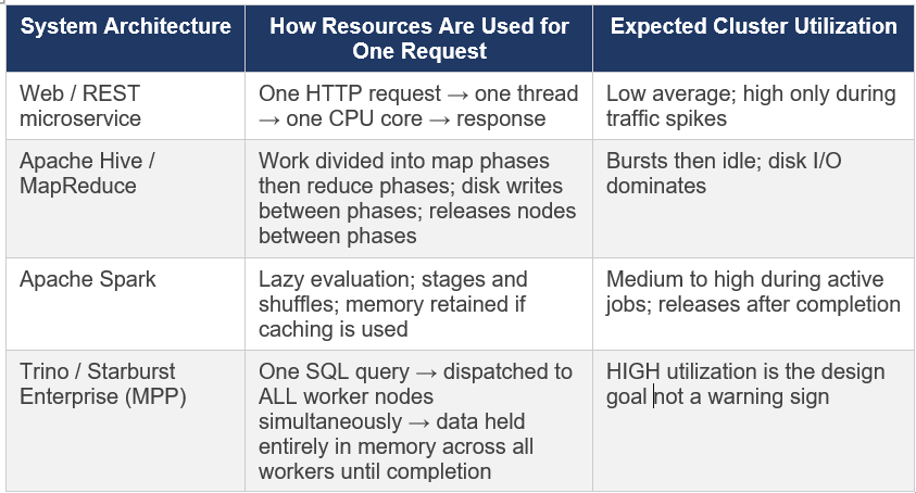
This is the single most important fact to internalise from this series. When a junior engineer sees 80% RAM across 25 workers and all CPUs busy, the correct interpretation is: the cluster is working exactly as designed. The questions to ask are not ‘why is utilization high?’ but rather ‘are queries completing successfully?’ and ‘are query latencies within acceptable ranges?’
2.2 Coordinator and Worker Architecture
A Trino/SEP cluster has two node types. The official Starburst documentation describes the coordinator as ‘the brain of a Trino installation’. Here is what each does in practice:
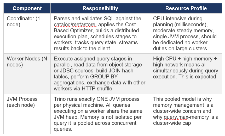
2.3 The Split — Trino’s Unit of Parallelism
The smallest unit of parallel work in Trino is called a split. For the Hive/Iceberg connector reading from object storage, a split typically corresponds to one file or a portion of a large file.
The number of splits available determines the maximum parallelism achievable for a scan:
1,000 splits across 25 workers × 32 threads each = all splits can be processed in one wave.
10 splits across 25 workers = most workers sit idle during the scan stage regardless of cluster size.
More splits is better up to the limit of available worker threads after that you get scheduling overhead without benefit
The implication for file management: Files smaller than roughly 8MB create very small splits with high scheduling overhead. Well-sized files (128MB to 1GB) produce appropriately-sized splits that keep all worker threads busy. This is why file compaction is one of the highest-leverage optimisations in Part 3 of this series.
2.4 Query Lifecycle — SQL to Results
Understanding the full execution path helps identify where slowdowns occur. A query travels through these stages:
1. Client submits SQL via HTTP POST to the Coordinator’s REST endpoint.
2. Coordinator parses the SQL and resolves table/column names against the Hive Metastore or Iceberg catalog this is where HMS slowness manifests.
3. The Cost-Based Optimizer (CBO) reads table statistics and builds a logical query plan, choosing join order, join distribution type, and aggregation strategy.
4. The physical planner converts the logical plan into a distributed execution plan composed of stages each stage is a set of tasks that can run on multiple workers in parallel.
5. The scheduler assigns available splits to workers and begins stage execution. Multiple stages can pipeline worker doesn’t wait for stage N to fully complete before starting stage N+1
6. Workers exchange intermediate data with each other via HTTP shuffle. This is the ‘network shuffle’ step that redistributes rows for GROUP BY keys and JOIN keys across workers.
7. The final output stage streams results back to the Coordinator, which returns them to the client.
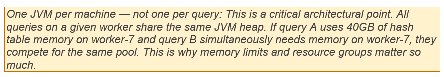
Trino does NOT write intermediate results to disk between stages. All data flows through memory. This is what makes it fast and why memory management is so consequential.
2.5 The Shared Hash Table — Why More CPU Helps Memory-Heavy Queries
During a JOIN operation, Trino builds a hash table from the build-side table (typically the smaller one) and streams the probe-side table through it looking up each row. This hash table is built once on each worker and shared across all probe threads on that worker it is not duplicated per thread.
The implication: adding more CPU cores to a JOIN-heavy query allows the probe phase to run faster, completing the query sooner and freeing the hash table memory. This is why high CPU utilization during JOIN operations is a sign the cluster is working efficiently, not a sign of resource waste.
Chapter 3: Cluster Sizing — The Right Foundation
Before any tuning is worth doing, the cluster needs to be correctly sized. Tuning a cluster that lacks sufficient headroom just moves the bottleneck around without solving it. The guidance from the 2020 Presto Training Series (Dain Sundstrom, Starburst) and production experience both point to the same starting strategy: start larger than you think you need, verify stability, then rightsize.
3.1 General Sizing Strategy
8. Build a cluster that has more capacity than your initial workload estimate. You need headroom to differentiate configuration problems from resource problems.
9. Verify stability first make sure queries complete without OOM errors and cluster behaviour is predictable.
10. Do NOT try to stabilize and performance-tune simultaneously they require different diagnosis approaches.
11. Measure the actual workload over time: peak memory per query, concurrent query count, CPU utilisation patterns.
12. Then rightsize downward reduce nodes or machine size until utilisation targets are met.
The most common failure pattern I’ve seen in Starburst deployments: teams provision a small cluster and immediately try to optimize it. Without headroom, you cannot tell whether slow queries are caused by configuration problems or by the cluster simply being too small. Always start bigger than you need.
3.2 CPU vs. Memory — Two Independent Dimensions
Trino has two independently scaling resource dimensions that behave very differently and require different responses when they become bottlenecks:
CPU — Controls Query Speed
More CPU cores → queries run faster. The relationship is approximately linear: doubling CPU halves query execution time.
CPU does NOT determine whether a query can run , only how fast it completes.
Running two identical queries concurrently with the same total CPU means each takes roughly 2x longer.
If queries are slow but completing without errors: the first thing to consider is whether you are CPU-constrained.
Memory — Controls Query Viability and Concurrency
Memory determines whether a query CAN run, not how fast it runs.
If a query requires 50GB of distributed hash table memory and your cluster only has 40GB available, the query fails, there is no ‘slow but succeeds’ for memory.
Memory is consumed by: JOIN hash tables, GROUP BY aggregation accumulators, ORDER BY sort buffers, window function frame data.
More memory increases the number of concurrent queries you can run and enables larger individual queries.
If queries are failing with EXCEEDED_LOCAL_MEMORY_LIMIT or EXCEEDED_GLOBAL_MEMORY_LIMIT errors: this is a memory problem, not a CPU problem
3.3 Fewer Bigger Machines vs. Many Smaller Machines
This is one of the most consequential sizing decisions. The guidance from both the Presto Training Series and production experience is clear: fewer, larger machines outperform many smaller ones for Trino workloads.
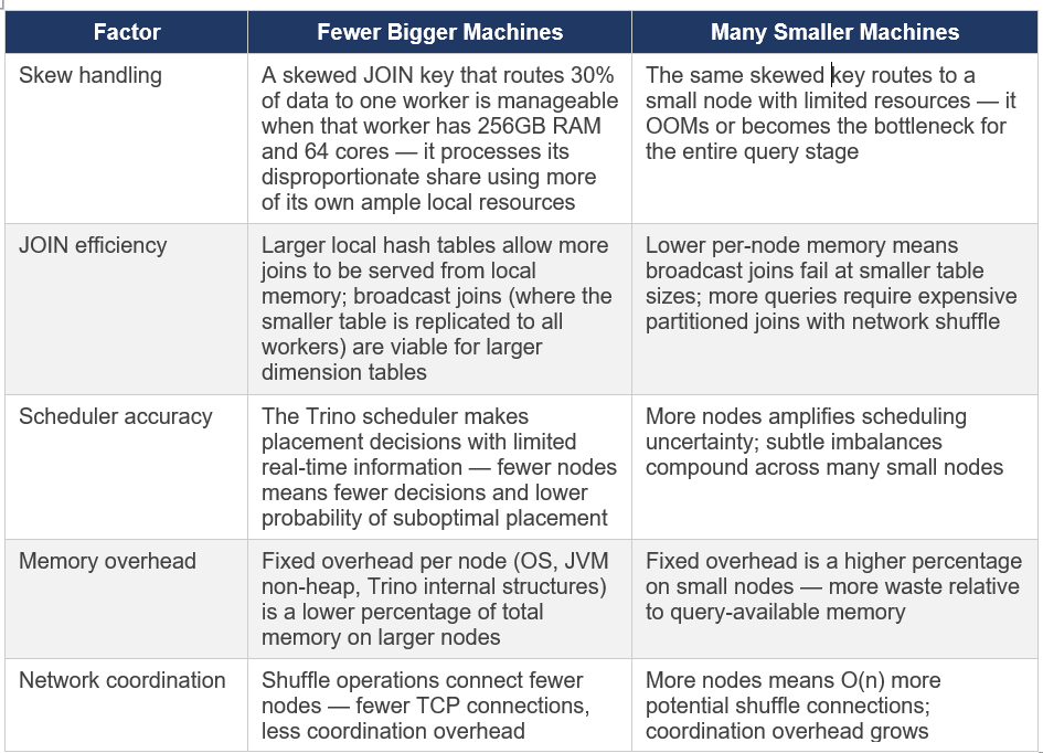
Production recommendation from experience: If choosing between 50 nodes with 64GB RAM each vs 25 nodes with 128GB RAM each for the same total cluster memory, choose the 25 larger nodes every time. The reduction in scheduling complexity, skew impact, and network overhead is significant and compounds over time.
3.4 Sizing for Concurrent Workloads
The hardest sizing question is not ‘how much does one query need?’ but ‘what is the peak concurrent demand?’. Some things I have learned:
Memory concurrency is additive: if query A needs 30GB cluster-wide and query B simultaneously needs 40GB, your cluster needs at least 70GB of query-accessible memory to run both at the same time.
CPU concurrency is time-sliced: the scheduler shares CPU time across concurrent queries. Adding queries increases latency for all queries rather than causing outright failures.
Peak concurrency, not average, determines minimum cluster size, size for your realistic P95 concurrent query memory demand.
Bigger clusters get a mix of query sizes that statistically even out. Small clusters are more vulnerable to a single heavy query consuming most available resources and causing other queries to queue.
3.5 Plan for Growth
Every Starburst deployment I have been involved with saw demand grow faster than expected. The platform is easy to use for SQL-familiar users, fast results encourage more queries, and federated access enables use cases teams never previously attempted. It is not unusual for query volume to double or even triple year over year once the platform is well-adopted. Build this into your sizing assumptions and your budget.
Chapter 4: Instance Type Selection — All Three Clouds
Starburst Enterprise is cloud-agnostic and fully supported on AWS, Azure, and GCP. You can deploy via native Kubernetes (EKS, AKS, GKE), directly on virtual machines using Starburst Admin, or via the respective cloud marketplaces. The right instance type for Trino/SEP workloads shares the same characteristics regardless of cloud: high memory-to-core ratio, high network bandwidth, and modern CPU platforms.
The guidance below is based on my experience selecting instance types for SEP workloads and on published instance specifications from each cloud provider. As cloud instance pricing and availability change frequently, always verify current pricing and availability in your region before committing.
4.1 General Principles Across All Clouds
Memory-optimized families are the first choice for JOIN-heavy and aggregation-heavy analytical workloads they give the highest memory per vCPU.
General-purpose balanced families work well when workloads are more scan-heavy or when memory per query is moderate.
Compute-optimized families are appropriate when workloads are CPU-bound with relatively small hash table sizes.
Network bandwidth matters: Starburst recommends a minimum 10 Gbps within the cluster; 25 Gbps is recommended for object storage access.
ARM/Ampere-based instances (Graviton on AWS, Ampere Altra on GCP and Azure) offer meaningful cost savings for the same workload — worth evaluating for production after benchmarking
4.2 Amazon Web Services (AWS)
The Presto Training Series (Starburst, 2020) originally provided AWS-centric guidance because that was the dominant cloud for Starburst workloads at the time. The recommendations remain relevant, though newer instance generations (m6i, r6i, m7i, r7i) offer better price-performance than the m5/r5 series shown in the original 2020 training.
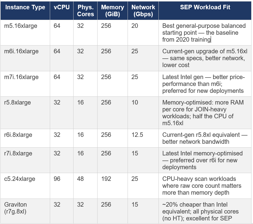
AWS note on vCPU vs physical cores: AWS instances use hyperthreading (2 threads per core). A 64-vCPU instance has 32 physical cores. Trino’s task.concurrency should be set to roughly 2x physical cores so 64 for a 32-core machine. For Graviton instances, each vCPU IS a full physical core, so task.concurrency can be set to the vCPU count directly.
4.3 Microsoft Azure
SEP is supported on Azure Kubernetes Service (AKS) and directly on Azure Compute Engine VMs via Starburst Admin. Azure’s instance families that match the workload profile for Trino are primarily in the E-series (memory-optimised) and D-series (general-purpose balanced).
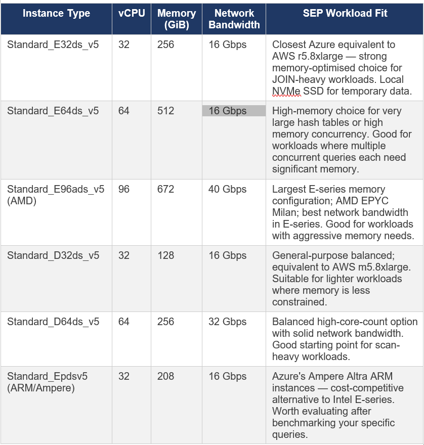
Azure-specific note: Azure’s E-series Esv5 instances (without ‘d’ in the name) do not have local temporary storage. The Edsv5 variants include local NVMe SSD. For SEP deployments where you might enable spilling (which I recommend against — see Part 2), you need the ‘d’ variants with local storage. For standard SEP use, either works, though local storage is useful for HMS and other auxiliary services.
Azure-specific considerations for SEP deployments:
Azure Data Lake Storage Gen2 (ADLS Gen2): SEP supports ADLS Gen2 natively as object storage via the Hive and Iceberg connectors. Use fs.native-azure.enabled=true in catalog configuration for the current native file system implementation.
Azure Kubernetes Service (AKS): The primary deployment mechanism for SEP on Azure. Use node pools with the instance types above dedicated to SEP coordinator and workers.
AKS Accelerated Networking: Ensure Accelerated Networking is enabled on all SEP node pool VMs this is critical for achieving the advertised network bandwidth figures
Azure Marketplace: SEP is available directly from the Azure Marketplace with PAYG licensing
4.4 Google Cloud Platform (GCP)
SEP is supported on Google Kubernetes Engine (GKE) and Google Compute Engine VMs. The official Starburst documentation lists GKE as the primary and fully certified deployment method on GCP. GCP’s machine naming convention is different from AWS and Azure: machines are described as ‘machine series’ (e.g., n2) + ‘machine type suffix’ (e.g., standard, highmem, highcpu).
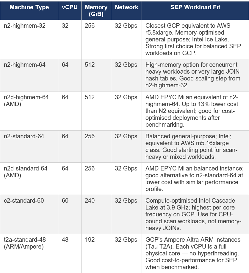
GCP-specific note on vCPUs: Unlike AWS, GCP’s standard (Intel/AMD) instances also use hyperthreading — each vCPU is one hardware thread. The Tau T2A (ARM/Ampere) is the exception: SMT (hyperthreading) is disabled, so each vCPU represents a full physical core. This matters for setting task.concurrency in Trino config (discussed in Part 2).
GCP-specific considerations for SEP deployments:
Google Cloud Storage (GCS): SEP reads from GCS via the native file system implementation. Use fs.native-gcs.enabled=true in your catalog configuration. The legacy GCS support is deprecated and will be removed in a future SEP version.
GKE Standard clusters: Recommended over Autopilot for SEP deployments that need precise control over node pool configuration and affinity rules.
Dataproc Metastore: Can serve as the Hive Metastore Service (HMS) for SEP catalogs on GCP — eliminates the operational overhead of managing your own HMS.
Sustained Use Discounts: GCP automatically applies sustained use discounts for N2 and N2D instances that run for most of the month — no upfront commitment required.
Committed Use Discounts (CUDs): Available for N2 and N2D — up to 55% savings for 3-year commitments
4.5 Multi-Cloud Comparison — Equivalent Instance Families
For teams operating across multiple clouds or evaluating which cloud to use for a new SEP deployment, this table maps roughly equivalent instance families across all three:
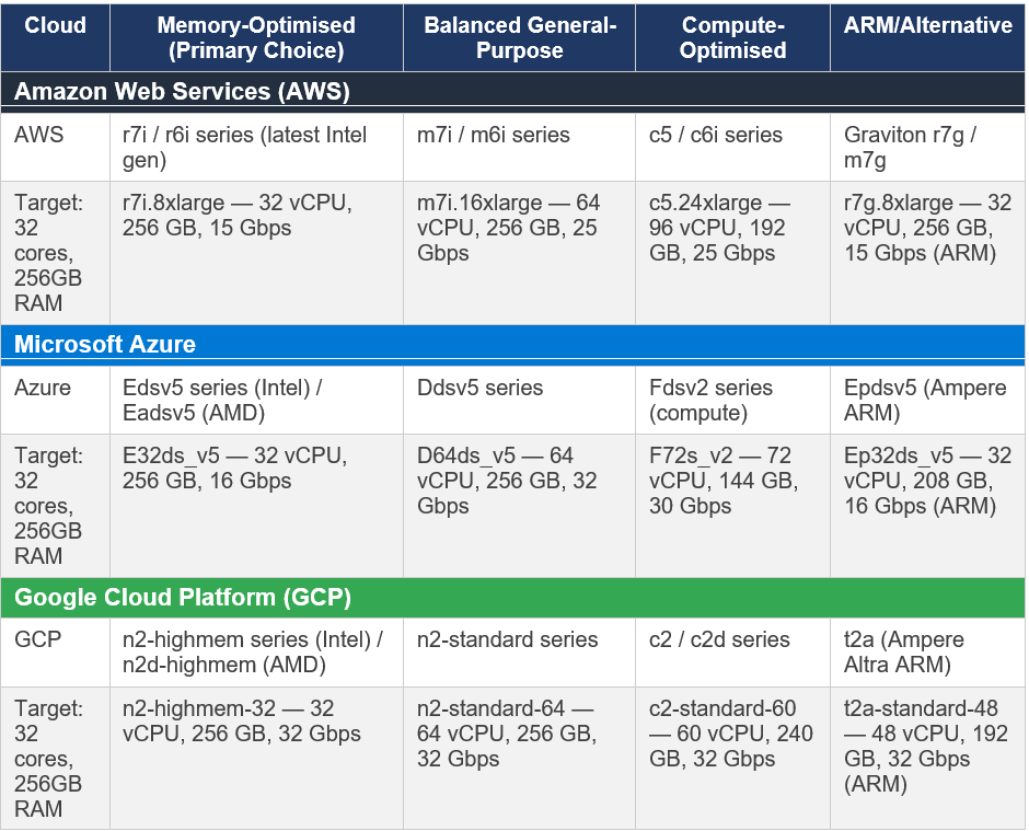
Important caveat on instance comparisons: Cloud pricing and availability change frequently. The instances listed above represent the general family recommendations as of early 2026. Always check current pricing in your specific region before making deployment decisions. For production workloads, benchmark your actual query mix on candidate instance types before committing — paper specs do not always translate to real-world Trino performance.
4.6 Kubernetes vs. VM Deployments
SEP supports both Kubernetes (K8s) and VM-based deployments. From a sizing perspective:
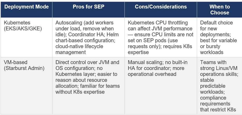
Kubernetes CPU limit note: The official Starburst Kubernetes configuration documentation explicitly warns about a known issue with Kubernetes CPU throttling. For SEP coordinator and worker pods, set CPU requests but do NOT set CPU limits. A hard CPU limit in Kubernetes causes JVM performance degradation due to CPU throttling even when the node has headroom. See docs.starburst.io/latest/k8s/sep-config-examples.html for the recommended values.yaml configuration.
Chapter 5: What High Utilisation Actually Means
Returning to where we started: the junior engineer’s observation of 80% RAM and fully utilised worker nodes. With the architectural understanding from this document, let me now give a proper answer.
5.1 The Correct Diagnostic Framework
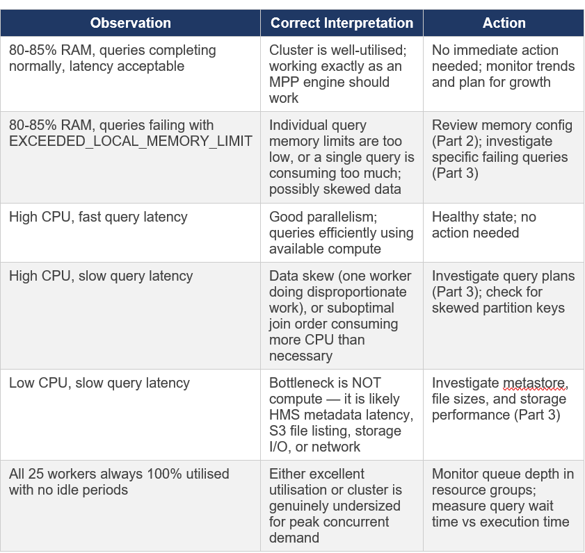
5.2 Metrics That Actually Matter
Rather than watching raw CPU or RAM percentages, monitor these metrics for a true picture of cluster health:
Query success rate: What percentage of submitted queries complete successfully? OOM errors show up here.
Query wait time (queue time): How long does a query spend waiting to be scheduled before execution begins? High queue time means the cluster is at capacity for concurrent queries.
Query execution time percentiles (P50, P95, P99): Are these stable or trending upward over time?
EXCEEDED_LOCAL_MEMORY_LIMIT error count: Queries failing with this error indicate memory pressure.
GC time ratio (via JMX): If GC time exceeds 10% of wall clock time on workers, memory pressure is affecting JVM performance.
Closing thought for Part 1: 80% RAM with 25 busy workers is exactly what a healthy, well-loaded MPP cluster looks like. The goal of a query engine is to efficiently use the resources you have provisioned. If utilisation were consistently low, that would mean you are over-provisioned and paying for idle resources. Monitor outcomes (query success, latency) not raw utilisation numbers.
References
Presto Training Series, Session 4: Cluster Sizing & Performance Tuning
Starburst Enterprise Documentation, SEP 477-e LTS (November 2025)
Series: Starburst Enterprise Performance Tuning | Part 1 of 3 | March 2026 | Validated against SEP 477-e LTS
will Continue with Part 2: Configuration Deep Dive : Memory, JVM & Concurrency